A Beginner’s Guide to Keras: Digit Recognition in 30 Minutes

Over the last decade, the use of artificial neural networks (ANNs) has increased considerably. People have used ANNs in medical diagnoses, to predict Bitcoin prices, and to create fake Obama videos! With all the buzz about deep learning and artificial neural networks, haven’t you always wanted to create one for yourself? In this tutorial, we’ll create a model to recognize handwritten digits.
We’ll use the Keras library for training the model in this tutorial. Keras is a high-level library in Python that is a wrapper over TensorFlow, CNTK and Theano. By default, Keras uses a TensorFlow backend by default, and we’ll use the same to train our model.
Artificial Neural Networks
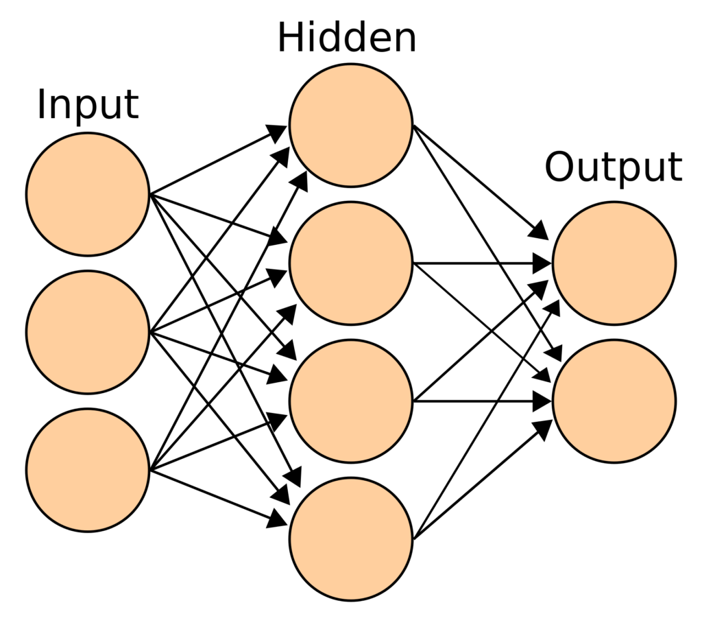
An artificial neural network is a mathematical model that converts a set of inputs to a set of outputs through a number of hidden layers. An ANN works with hidden layers, each of which is a transient form associated with a probability. In a typical neural network, each node of a layer takes all nodes of the previous layer as input. A model may have one or more hidden layers.
ANNs receive an input layer to transform it through hidden layers. An ANN is initialized by assigning random weights and biases to each node of the hidden layers. As the training data is fed into the model, it modifies these weights and biases using the errors generated at each step. Hence, our model “learns” the pattern when going through the training data.
Convoluted Neural Networks
In this tutorial, we’re going to identify digits — which is a simple version of image classification. An image is essentially a collection of dots or pixels. A pixel can be identified through its component colors (RGB). Therefore, the input data of an image is essentially a 2D array of pixels, each representing a color.
If we were to train a regular neural network based on image data, we’d have to provide a long list of inputs, each of which would be connected to the next hidden layer. This makes the process difficult to scale up.
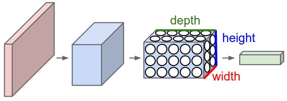
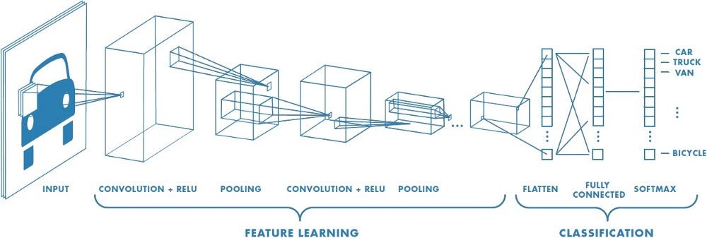
In a convoluted neural network (CNN), the layers are arranged in a 3D array (X-axis coordinate, Y-axis coordinate and color). Consequently, a node of the hidden layer would only be connected to a small region in the vicinity of the corresponding input layer, making the process far more efficient than a traditional neural network. CNNs, therefore, are popular when it comes to working with images and videos.
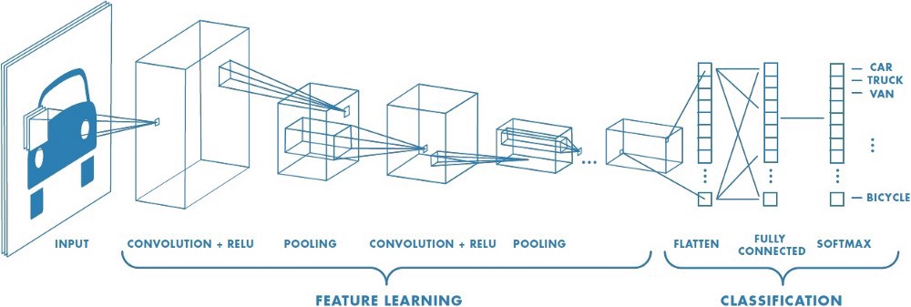
The various types of layers in a CNN are as follows:
- convolutional layers: these run input through certain filters, which identify features in the image
- pooling layers: these combine convolutional features, helping in feature reduction
- flatten layers: these convert an N-dimentional layer to a 1D layer
- classification layer: the final layer, which tells us the final result
Let’s now explore the data.
Explore MNIST Dataset
As you may have realized by now that we need labelled data to train any model. In this tutorial, we’ll use the MNIST dataset of handwritten digits. This dataset is a part of the Keras package. It contains a training set of 60,000 examples, and a test set of 10,000 examples. We’ll train the data on the training set and validate the results based on the test data. Further, we’ll create an image of our own to test whether the model can correctly predict it.
First, let’s import the MNIST dataset from Keras. The .load_data() method returns both the training and testing datasets:
from keras.datasets import mnist

(x_train, y_train), (x_test, y_test) = mnist.load_data()
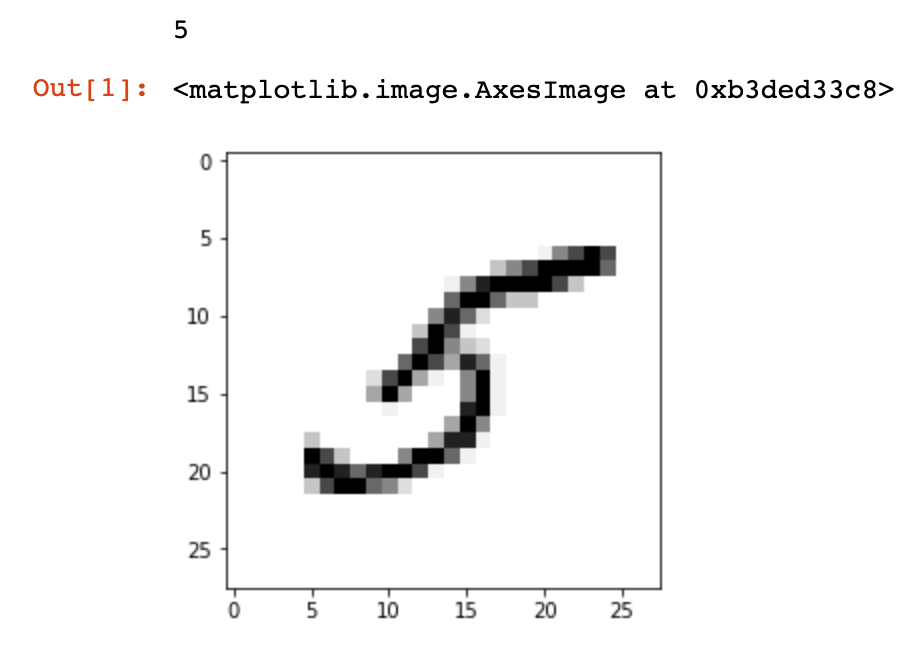
Let’s try to visualize the digits in the dataset. If you’re using Jupyter notebooks, use the following magic function to show inline Matplotlib plots:
%matplotlib inline
Next, import the pyplot module from matplotlib and use the .imshow() method to display the image:
import matplotlib.pyplot as plt

image_index = 35
print(y_train[image_index])
plt.imshow(x_train[image_index], cmap='Greys')
plt.show()
The label of the image is printed and then the image is displayed.
Let’s verify the sizes of the training and testing datasets:
print(x_train.shape)
print(x_test.shape)
Notice that each image has the dimensions 28 x 28:
(60000, 28, 28)
(10000, 28, 28)
Next, we may also wish to explore the dependent variable, stored in y_train. Let’s print all labels till the digit that we visualized above:
print(y_train[:image_index + 1])
[5 0 4 1 9 2 1 3 1 4 3 5 3 6 1 7 2 8 6 9 4 0 9 1 1 2 4 3 2 7 3 8 6 9 0 5]
Cleaning Data
Now that we’ve seen the structure of the data, let’s work on it further before creating the model.
To work with the Keras API, we need to reshape each image to the format of (M x N x 1). we’ll use the .reshape() method to perform this action. Finally, normalize the image data by dividing each pixel value by 255 (since RGB values can range from 0 to 255):
# save input image dimensions
img_rows, img_cols = 28, 28

x_train = x_train.reshape(x_train.shape[0], img_rows, img_cols, 1)
x_test = x_test.reshape(x_test.shape[0], img_rows, img_cols, 1)

x_train /= 255
x_test /= 255
Next, we need to convert the dependent variable in the form of integers to a binary class matrix. This can be achieved by the to_categorical() function:
from keras.utils import to_categorical
num_classes = 10

y_train = to_categorical(y_train, num_classes)
y_test = to_categorical(y_test, num_classes)
We’re now ready to create the model and train it!
Design a Model
The model design process is the most complex factor, having a direct impact on the performance of the model. For this tutorial, we’ll use this design from the Keras documentation.
To create the model, we first initialize a sequential model. It creates an empty model object. The first step is to add a convolutional layer, which takes the input image:
from keras.models import Sequential
from keras.layers import Dense, Dropout, Flatten, Conv2D, MaxPooling2D

model = Sequential()
model.add(Conv2D(32, kernel_size=(3, 3),
     activation='relu',
     input_shape=(img_rows, img_cols, 1)))
A relu activation stands for “Rectified Linear Units”, which takes the max of a value or zero. Next, we add another convolutional layer, followed by a pooling layer:
model.add(Conv2D(64, (3, 3), activation='relu'))
model.add(MaxPooling2D(pool_size=(2, 2)))
Next, we add a “dropout” layer. While neural networks are trained on huge datasets, a problem of overfitting may occur. To avoid this issue, we randomly drop units and their connections during the training process. In this case, we’ll drop 25% of the units:
model.add(Dropout(0.25))
Next, we add a flattening layer to convert the previous hidden layer into a 1D array:
model.add(Flatten())
Once we’ve flattened the data into a 1D array, we can add a dense hidden layer, which is normal for a traditional neural network. Next, add another dropout layer before adding a final dense layer which classifies the data:
model.add(Dense(128, activation='relu'))
model.add(Dropout(0.5))
model.add(Dense(num_classes, activation='softmax'))
The softmax activation is used when we’d like to classify the data into a number of pre-decided classes.
Compile and Train Model
In the model design process, we’ve created an empty model without an objective function. We need to compile the model and specify a loss function, an optimizer function, and a metric to assess model performance.
We need to use a sparse_categorical_crossentropy() loss function in case we have an integer-dependent variable. For a vector-based dependent variable like a ten-size array as the output of each test case, use categorical_crossentropy. In this example, we’ll use the adam optimizer. The metric is the basis for the assessment of our model performance, though it’s only for us to judge and isn’t used in the training step:
model.compile(loss='sparse_categorical_crossentropy',
      optimizer='adam',
      metrics=['accuracy'])
We’re now ready to train the model using the .fit() method. We need to specify an epoch and batch size when training the model. An epoch is one forward pass and one backward pass of all training examples. A batch size is the number of training examples in one forward or backward pass.
Finally, save the model once the training is complete to use its results at a later stage:
batch_size = 128
epochs = 10

model.fit(x_train, y_train,
          batch_size=batch_size,
          epochs=epochs,
          verbose=1,
          validation_data=(x_test, y_test))
score = model.evaluate(x_test, y_test, verbose=0)
print('Test loss:', score[0])
print('Test accuracy:', score[1])
model.save("test_model.h5")
When we run the code above, the following output is shown as the model runs. It takes about ten minutes in a 2018 Macbook Air running Jupyter notebooks:
Train on 60000 samples, validate on 10000 samples
Epoch 1/10
60000/60000 [==============================] - 144s 2ms/step - loss: 0.2827 - acc: 0.9131 - val_loss: 0.0612 - val_acc: 0.9809
Epoch 2/10
60000/60000 [==============================] - 206s 3ms/step - loss: 0.0922 - acc: 0.9720 - val_loss: 0.0427 - val_acc: 0.9857
...
Epoch 9/10
60000/60000 [==============================] - 142s 2ms/step - loss: 0.0329 - acc: 0.9895 - val_loss: 0.0276 - val_acc: 0.9919
Epoch 10/10
60000/60000 [==============================] - 141s 2ms/step - loss: 0.0301 - acc: 0.9901 - val_loss: 0.0261 - val_acc: 0.9919
Test loss: 0.026140549496188395
Test accuracy: 0.9919
At the end of the final epoch, the accuracy of the test dataset is 99.19%. It’s difficult to comment on how high the accuracy needs to be. For a test run, accuracy over 99% is very good. However, there’s a lot of scope for improvement by tweaking the model parameters. There’s a submission from a digit recognizer contest on Kaggle that reached 99.7% accuracy.
Test with Handwritten Digits
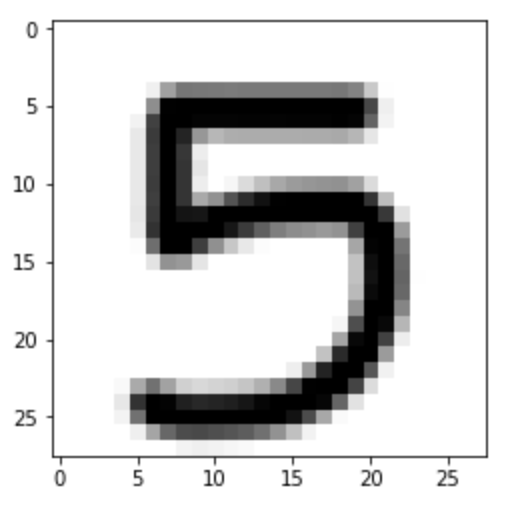
Now that the model is ready, let’s use a custom image to assess the performance of the model. I’ve hosted a custom 28×28 digit on Imgur. First, let’s read the image using the imageio library and explore how the input data looks:
import imageio
import numpy as np
from matplotlib import pyplot as plt

im = imageio.imread("https://i.imgur.com/a3Rql9C.png")
Next, convert the RGB values to grayscale. We can then use the .imshow() method as explored above to display the image:
gray = np.dot(im[...,:3], [0.299, 0.587, 0.114])
plt.imshow(gray, cmap = plt.get_cmap('gray'))
plt.show()
Next, reshape the image and normalize the values to make it ready to be used in the model that we’ve just created:
# reshape the image
gray = gray.reshape(1, img_rows, img_cols, 1)

# normalize image
gray /= 255
Load the model from the saved file using the load_model() function and predict the digit using the .predict() method:
# load the model
from keras.models import load_model
model = load_model("test_model.h5")

# predict digit
prediction = model.predict(gray)
print(prediction.argmax())
The model correctly predicts the digit shown in the image:
5
Final Thoughts
In this tutorial, we created a neural network with Keras using the TensorFlow back end to classify handwritten digits. Although we reached an accuracy of 99%, there are still opportunities for improvement. We also learned how to classify custom handwritten digits, which were not a part of the test dataset. This tutorial, however, has just scratched the surface of the artificial neural networks field. There are endless uses for neural networks that are only limited by our imagination.
Are you able to improve the accuracy of the model? What other techniques can you think of using? Let me know on Twitter.


